3: Spatially Enabled Relational Databases

3.2 In-Class Exercise: Building the IFRI Spatial Relational Database using PostGIS

Introduction

In this class exercise, we will turn back to the International Forestry Resources and Institutions (IFRI) relational database we worked on earlier. But in today’s work, we will build a spatially-explicit relational database using Postgres, PostGIS, and QGIS.

Recall the simple relational database we designed previously (Figure 1).

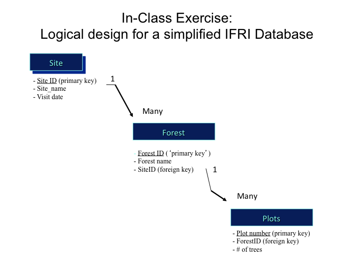
The overall plan for this in-class exercise will be to do the following:

Build a new IFRI QGIS project and connect to our town and landsat image data
Import a shapefile polygon of one Forest area (MtToby) into PostGIS to create a spatially-explicit Forest layer
Select out the towns that cover MtToby in QGIS to produce a new Site layer
Create a new point layer for the Forest Plots 5. Set up our relational primary and foreign keys and enter some trial data into the database (attribute tables)
Run a multiple-table query to answer a question
How could you have queried the forest plots that are in the Mt Toby boundary without setting up the 1-to-many relationship?
Take a screen shot of your final QGIS screen and upload it to Moodle under Week 3 to document that you completed the exercise.

Let’s begin!

————-

To start, create a Week_3 folder on your computer hard disk to store your work.

Task 1) Set up our base QGIS IFRI project

Open up QGIS Project and a new blank map. If you have residual connections to previous exercise data in your Browser (like the Boundless nyc data), consider removing them (right click, delete).

Note the “Render” and the default project coordinate system used at the bottom right of your QGIS map screen. In our instance, it defaults to “EPSG: 4326”.

Do a Google Search on EPSG: 4326. You’’ll find information noting that this is a reference to WGS84.

Question 1: What does that mean? For the answer, see the end of this exercise.

Question 2: What kind of distortion occurs using that coordinate system discussed in Question 1?

Here’s a little detail that is kind of confusing but relates to the Boundless readings you did earlier and is important to understand. Recall in the Boundless readings there was a discussion about SRID — it stands for Spatial Reference System Identifier. Recall that the SRID is a unique value that is associated with a particular spatial coordinate system and there are thousands of them.

In QGIS, they use EPSG rather than SRID. EPSG stands for the European Petroleum Survey Group and they have numbers to reference various spatial coordinate systems. So the EPSG number 4326 references the geographic coordinate system (latitude and longitude) using WGS84 as its datum and no projection.

On to working with our data.

Add a UMass Web Feature Service (WFS) using our Geoserver. Do you remember how to do this? We did this in the first exercise “Exploring Spatial Data Models using QGIS”. The information you need to make that connection is:

Name: UMass WFS (you can call this whatever you want, actually) URL: http://nrcwg01.eco.umass.edu:8080/geoserver/massachusetts/wfs

Double-click on the umass WFS “towns” layer to get it added to your Layers list in QGIS.

Now look at the “Render” and the coordinate system at the bottom right of your screen. What does it say now?

By bringing in our first layer (Umass FMS Towns), the project coordinate system took on the projection used in that layer, EPSG:26986.

Before we move on, check out the QGIS Project Properties (Project menu, Project Properties). You should see near the bottom that it says “Selected CRS” (CRS stands for Coordinate Reference System) and it should be referencing “NAD83/Massachusetts Mainland”

Question 3: Can you interpret that? What is that telling you (see the answer below)?

Before we close the Project Properties screen, click on “Enable ‘on the fly’ CRS transformation” (Figure 1A). As you probably know, this will allow QGIS to display or overlay layers with different coordinate systems on top of each other using a behind-the-scenes conversion algorithm.

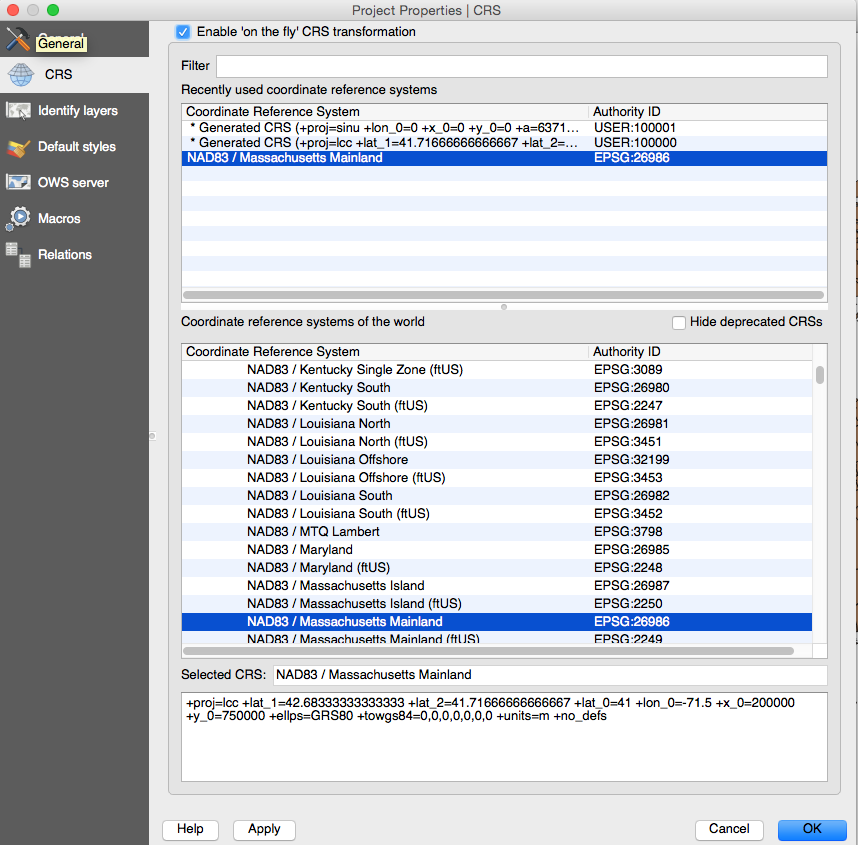
Now let’s get the background Landsat image.

Connect to the Umass Web Mapping Service (WMS). Again, we first used this function in the first exercise referenced above. Like the WFS above, we need the following information to create the connection:

Name: UMass WMS (again, this can be called whatever you want to call it) URL: http://nrcwg01.eco.umass.edu:8080/geoserver/wms?

Once the connection is established in your QGIS Browser, double-click on the “Landsat-image” layer to load it into your QGIS layers. Reorder or move down the Landsat image so the towns boundaries sit on top of the landsat image. Change the symbology of the towns layer so the fill color is off and the boundary color is easily seen on top of the Landsat image (Figure 2).

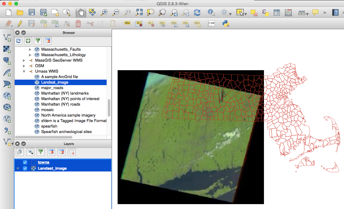
Save your QGIS project. Call it something like “Yourname_IFRI” and store it in some exercise folder on your computer.

Task 2: Import a shapefile polygon boundary of one Forest area (MtToby) into PostGIS to create a spatially-explicit Forest layer

First, we need to create a boundary layer of the one forest property we will work with in this exercise: Mt Toby.

Get the MassGIS Openspace layer. We assume you’ve had some experience with MassGIS. Go to that website and find the “Openspace” shapefile and download it to your exercise folder. Unzip it. In that folder there is an OPENSPACE_POLY.shp. Add that to your QGIS project and temporarily, turn off the display of the towns and landsat image. Your QGIS map should look like Figure 3, below.

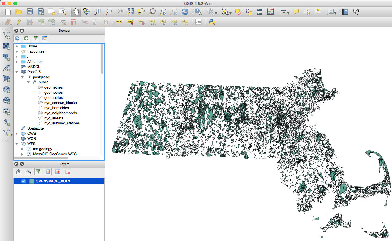
Using QGIS’ Select by Expression function ( ) to run a query that selects just the polygons in the OpenSpace _poly layer where

( "SITE_NAME" = 'Mount Toby State Forest' ) OR ( "SITE_NAME" = 'Mt Toby Conservation Area' )

As shown in Figure 5 below.

Press the Select button. Several polygons will be selected (Figure 6).

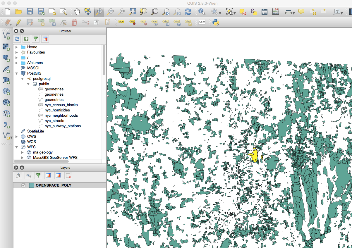
We’ve now selected the forested areas that are part of our IFRI research study. Let’s save the selected features to an ESRI Shapefile to your exercise folder hard disk.

Under the QGIS main menu, Layer option, press “Save As”.
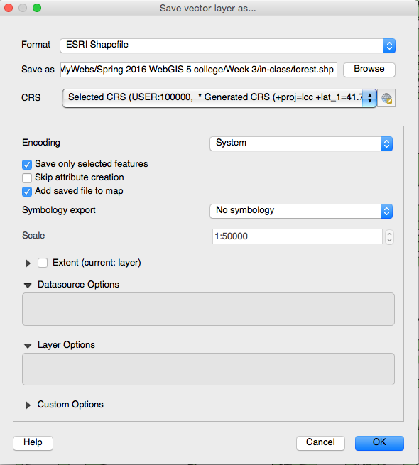
Under Format, choose: “ESRI Shapefile” but notice all the other format types available, some of which were discussed in the previous reading (Figure 7).
Next to Save as, press the “Browse” button and save the selected polygons as a new shapefile called “forest” (for our Forest Spatial Layer shown in the relational database design in Figure 1). Save it in your exercise folder on your hard disk.
Before you press OK, make sure you select “Save only Selected Features” and “Add saved file to map” (Figure 8).
Press OK, and you should see a new shapefile displayed in your QGIS Layers window called “forest” (Figure 9).

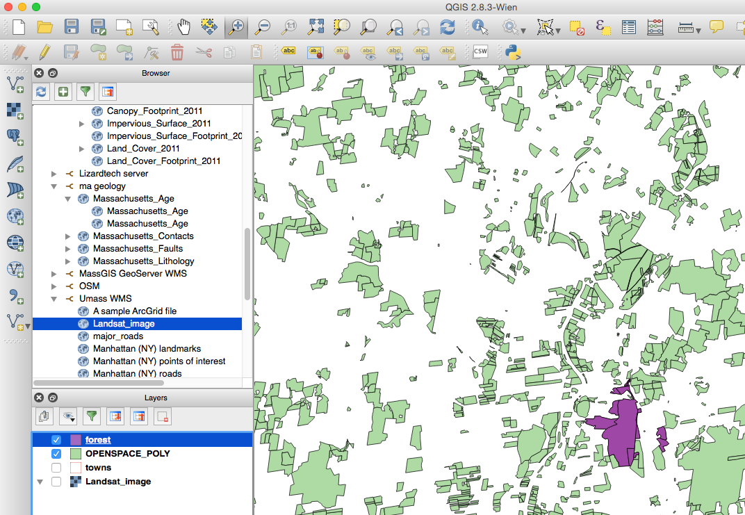
Open up the Forest attribute table. Note that there are actually 19 polygons that make up the Mt Toby forest, and there are a number of different owners of various parcels. This simulates the “many forest” side of the database design in Figure 1.

Up until now we’ve been working with either Web Service data or the proprietary data format Shapefile. Let’s now begin to build our IFRI Study PostGIS relational database. Hopefully you recall the steps from the pre-class reading exercise. See if you can create a database named IFRI in PostGIS that is spatially enabled. But if you can’t see Answer 4 below for the steps. Remember, you do this part in pgAdmin and not in QGIS!

Once you do that, you should be able to connect to your database with QGIS as described in Chapter 3.1.

Now, let’s work on getting the Forest shapefile imported into this database. QGIS has a Database Manager that we’ll use to convert the forest shapefile into a PostGIS data set.

In QGIS Desktop, menu Database > DB Manager > DB Manager.
Open the list item PostGIS.
Click on the connection to your database that you created previously.
Click on the button Import layer/file.
In the dialog Import vector layer, in the menu Input, choose the layer to import from those already brought into QGIS, e.g. forest (you can also click the button … to load another file);
Click the button Update options to copy the Input name to the Table name.
Click the button OK.

If you are here, you hopefully were successful importing the forest shapefile into the IFRI postGIS database. Now, display it in QGIS.

See if you can figure out the steps yourself. If you have trouble, see Answer 5 below.

Hopefully at this point you are successful and you have the forest layer in your PostGIS database and you are displaying it in QGIS! We have our first component of our IFRI database — the Forest layer!

Task 3: Select out the towns that cover MtToby in QGIS to produce a new Site layer

So now that we have a Forest layer for our IFRI database, now let’s create a layer for our Site component of the database (see Figure 1). In this case, a “research site” here in the US we’ll call a town or towns where the forests reside.

Let’s use the Umass Towns WFS layer to see what town(s) the Mt Toby property resides in. Turn off all layers except for the forest layer and the towns layer as shown in Figure 10.

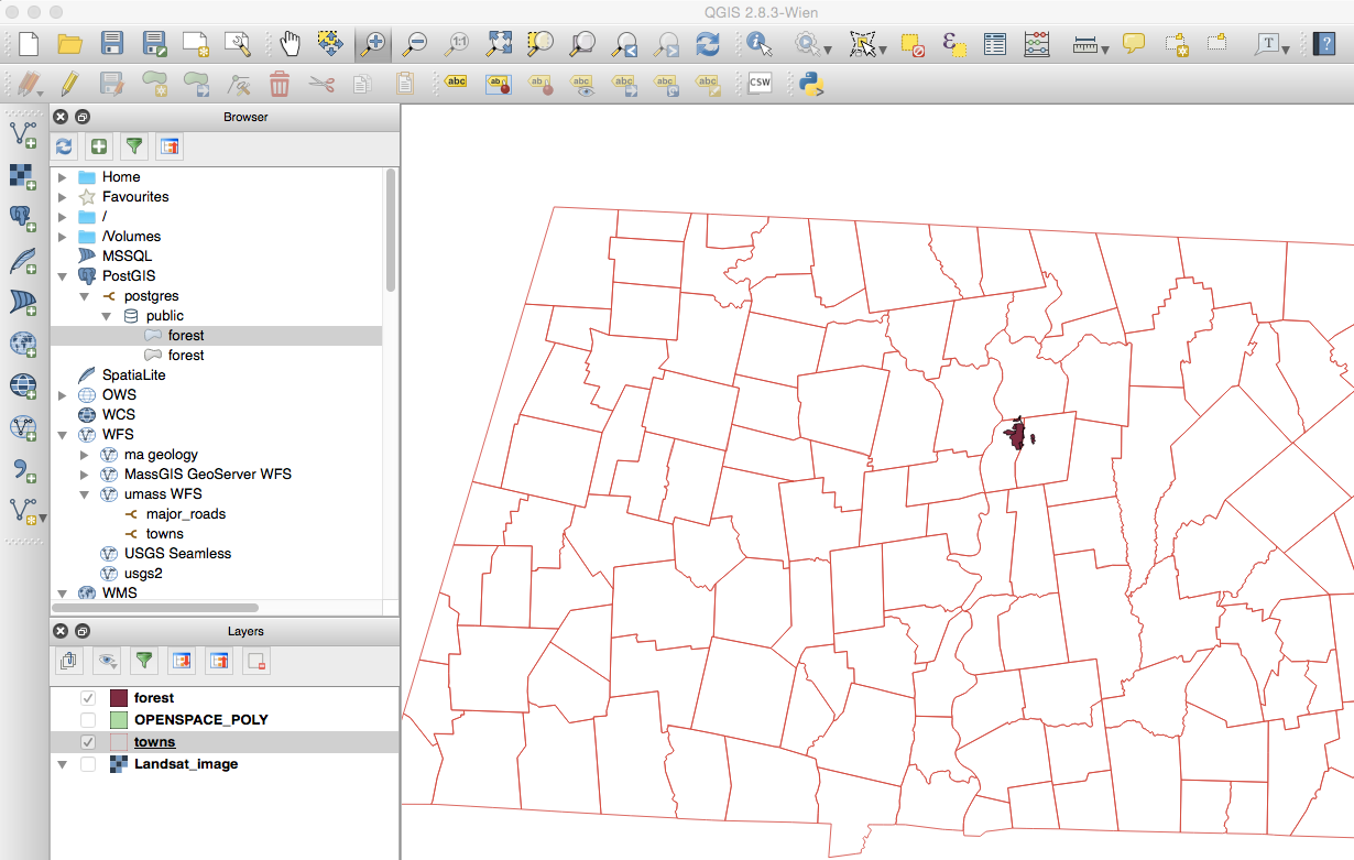
Using QGIS, see if you can can figure out steps to create a new shapefile that includes just the town boundaries that the Mt Toby forest resides in (the answer should be three polygons). But for the study site polygon, what we want to produce is ONE polygon representing the outer boundary of the towns that the Mt Toby forest resides in. So see if you can, without looking at our answer, figure out the steps to do the following:

select the towns that Mt Toby falls in;
save these selected polygons as a shapefile called ‘mttoby_towns’
merge the three polygons to create one larger polygon
Save that as a “Site” shapefile
Store that new Site shapefile in the IFRI PostGIS database
Add that new PostGIS layer to your QGIS Layers and map.

If you get stuck and need to see one method, we describe our steps below to Answer 6.

If all went as planned, you should now have a single Site polygon that encompasses the areas taken up by the towns of Montague, Sunderland, and Leverett. At this point, we no longer need the shapefiles since the Forest and Site layers reside in our IFRI database in PostGIS. In QGIS, right click and remove the work layers we no longer need: Openspace, mt_toby_town and the site shapefiles. Your QGIS system should look something like the future below with the forest and site coming from the PostGIS IFRI database.

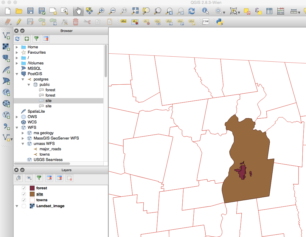
Thinking back to our Forest layer and our database design in Figure 1, we now have the situation where we have one research SITE (made up of the three towns of Montague, Sunderland and Leverett), and within this SITE we have several FOREST polygons, all of which are parts of Mt Toby, but are owned by different organizations. Conceptually, we have a 1 site with many forests situation now.

Task 4) Create a new point layer for the Forest Plots

With two of our three spatial layers in our IFRI PostGIS RDBMS built, we now need to turn to the third table in our ER diagram (Figure 1): the forest Plots table.

The idea of the Plots table is this: It would be a point layer where biologists would create a center point with a 10 meter circle and then sample all the vegetation that falls within those circles or ‘forest plots.’ These are one method that foresters or biologists use to inventory vegetation in a forested area.

Right now, we have no forest plots mapped. One way to do this would be to go out and GPS some random locations or follow some kind of transect sampling method. Another way, which we’ll do here, would be to have the GIS system create a point layer of randomly placed points.

See if you can figure out how you can make QGIS create a point layer of randomly placed points within the Mt Toby Forest polygon with a GID = 10 (Figure 12).

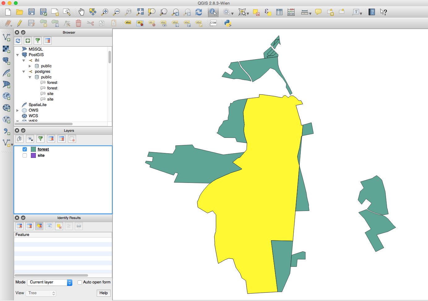
Try to do it yourself. If you can’t figure it out, look down at Answer 7 below. (Two Hints: (1) You need to first select out the polygon with GID = 1 and save it as its own layer; and (2) there is a QGIS command that will do the random point placement very easily for you. Don’t digitize the points yourself!).

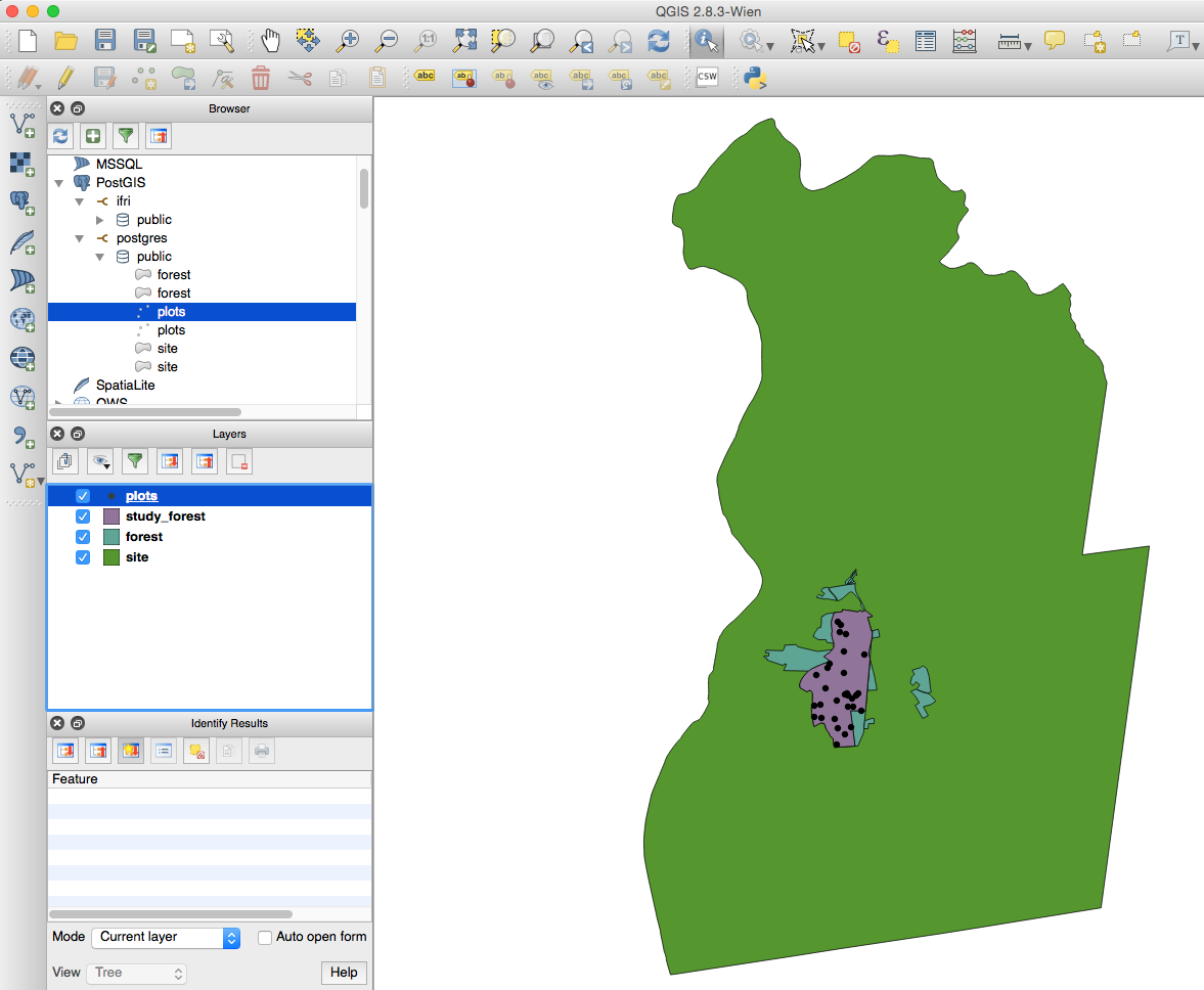
Once you have the random plots shapefile created, go through the process of adding it to your PostGIS IFRI database and bring that into your QGIS Layers list. Remove the old shapefile versions.

We now should have all three of our IFRI database layers: Site, Forest and Plots. Your QGIS map should look similar to the Figure below.

Task 5) Set up our relational primary and foreign keys and enter some trial data into the database (attribute tables)

So first we need to make up some ‘fake’ forest plot data. Since you are probably just learning how to use QGIS (but probably have experience with another GIS package), see if you can figure out how to edit the Plots table and add these columns (following our simple ER design in Figure 1):

Plot_number(integer, auto increment)

ForestID

Num_trees (diameter at breast height)

After you’ve created the fields, enter the following data into your plots attribute table:

plot_num, forestID, Num_trees

1,1,10

2,1,5

3,1,7

4,1,14

5,1,3

6,1,8

7,1,0

8,1,2

9,1,10

If you aren’t sure how to do this, go down and review Answer 8 below.

So now we have some data in our plots table. Now let’s enter the primary and foreign keys in our Site and Forest table to set up our relational database again. Look back to our design in Figure 1.

In the Site attribute table enter these two fields:

Site_ID (primary key, integer))

Site_name (text, fixed length, 30)

In the Forest attribute table we need:

Forest_ID (primary key, integer)

Forest_name (text. fixed length, 50)

Site_ID (foreign key, integer)

Follow the same steps you did above to add fields to plot to add the fields in these tables.

Once you have that done, enter the relevant data to set up the relationships:

Site_Id, Site_Name

1, Western MA

In the Forest Table, remember the only forest polygon we are working with is gid = 9. For THAT ROW ONLY enter this data:

Forest_ID, Forest_Name, Site_ID

1,Mount Toby,1

Save your edits.

In case you didn’t read the Answer 8 below, you could have done this portion of the exercise with either tables in QGIS, or using pgAdmin to work with the tables.

Task 6) Run a multiple-table query to answer a question

So now we are in a position to try and query all of the data associated with Sites, Forests and Plots. That is, do a relational database join query.

But before we do this, there are too many fields in Forest right now that we don’t need. In QGIS, open up the Forest table, click on the “Delete Attributes” icon, and delete the middle 10 or so fields that we didn’t enter. You need to edit the forest table in order to do this. Turn editing off when done.

Recall from our Week 2 exercise with pgAdmin that we used the Graphical Query Builder to run a query that pulled data from multiple tables together.

Run the query: “Show me all of the forest plot records for Site 1, Forest 1”

If you don’t know how to do this, review Answer 9, below.

Task 7) How could you have queried the forest plots that are in the Mt Toby boundary without setting up the 1-to-many relationship?

See Answer 10 if you aren’t sure.

Task 8) Take a screen shot of your final QGIS screen, name it “your last name Week 3” and upload it in Moodle Week 3 for proof that you completed this exercise.

ANSWERS TO QUESTIONS

Question 1. WGS84 means that the default coordinate system for QGIS is a Latitude\Longitude coordinate system using the World Geodetic System 1984 which is is the datum, with a reference ellipsoid. So QGIS defaults to using a world, lat\long system.

Question 2. Mapping in Lat\Long coordinates means that distortion occurs in all four types: Shape, Area, Distance and Direction.

Question 3. NAD83 is the datum used — North American Datum 1983. Massachusetts Mainland is referring to the State Plane Projection for Massachusetts (the mainland part of Massachusetts). Hopefully you remember this from earlier GIS classes!

Answer 4. Setting up an IFRI PostGIS database.

First, use pgAdmin, to create the IFRI database.

The steps to do this are described in the Boundless Creating a Spatial Database reading (http://workshops.boundlessgeo.com/postgis-intro/creating_db.html). But basically they are:

start up pgAdmin
create the ifri database by right clicking on the Databases under postgresql and naming it “IFRI” with an owner of “postgres”
Under the IFRI database, choose use the public schema. Use the SQL query tool to run the “CREATE EXTENSION postgis;”
run the “SELECT postgis_full_version();” query to verify that it is operational.

Answer 5. Steps to viewing PostGIS layer data in QGIS

In Browser, right click on the PostGIS option
Fill in the following information: Name - postgres (or you could name it something else); Host - ‘localhost’ (no quotes); Database - IFRI; Username - postgres; password - postgres. Test the connection. Hopefully successful! Click OK. *You should see ‘postgres’ or whatever you named the PostGIS connection appear below PostGIS in the browser. Open up the little triangles and navigate down to the database “public.” You should see ‘forest’ as a layer listed. Click on it, and a QGIS window ‘Coordinate Reference System Selector’ will appear. It will have the CRS from the shapefile (Massachusetts Mainland, NAD83). Hit OK. You should see the PostGIS forest layer appear in your QGIS Layers window and on the map.
Check out the properties for the forest layer. Look under the General tab. The layer source will be referring to the PostGIS database and notice the type is a ‘multipolygon’. The previous Boundless readings should be useful here in understanding this. Return up to the exercise.

Answer 6. Steps to selecting out the towns that contain the Mt Toby forest polygons using QGIS

To select out the three towns that have the mt toby forest in it and save them to a shapefile:

go to QGIS menu, Vector, Research Tools, Select by Location
Select features in towns, that intersect features in forest. Include input features that intersect the selection features. Create new selection. OK.
Three towns should be selected. You can see which ones (their names) if you open the attribute table for towns and press “show selected features” at the bottom. The towns are: Montague, Sunderland and Leverett.
Layer menu item, Save as, Format ESRI Shapefile, CRS keep as Mass Mainland. Browse to store in your exercise folder. Output as “mt_toby_towns.shp”. Make sure you choose “save only selected features.” Press OK.

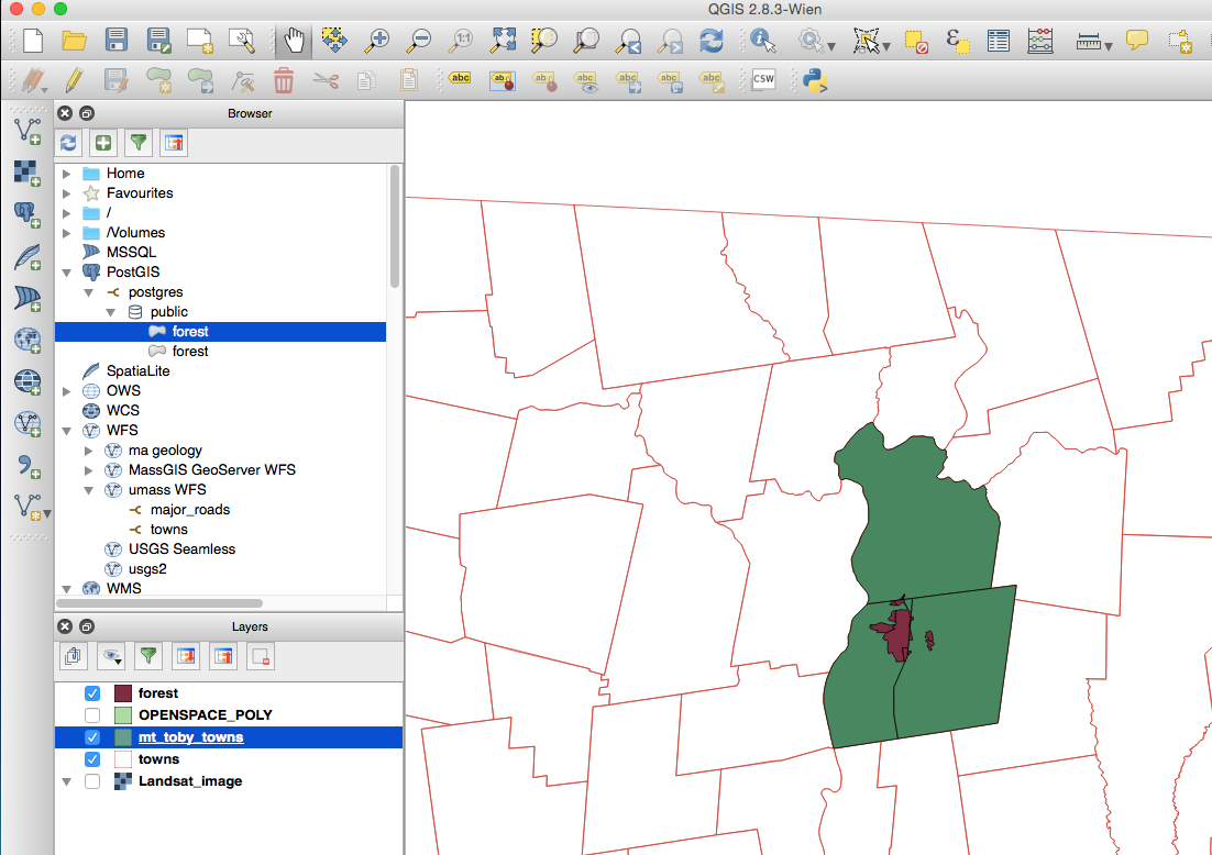
One way to merge the three polygons to create one larger polygon:

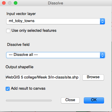
QGIS menu, Vector, Geoprocessing tools, Dissolve
Input vector layer: Mt_toby_towns; Dissolve field: Dissolve all; output to your exercise folder as “site” shapefile

The result will be a dissolve of the three polygons into one polygon that contains their area as shown in the figure below.

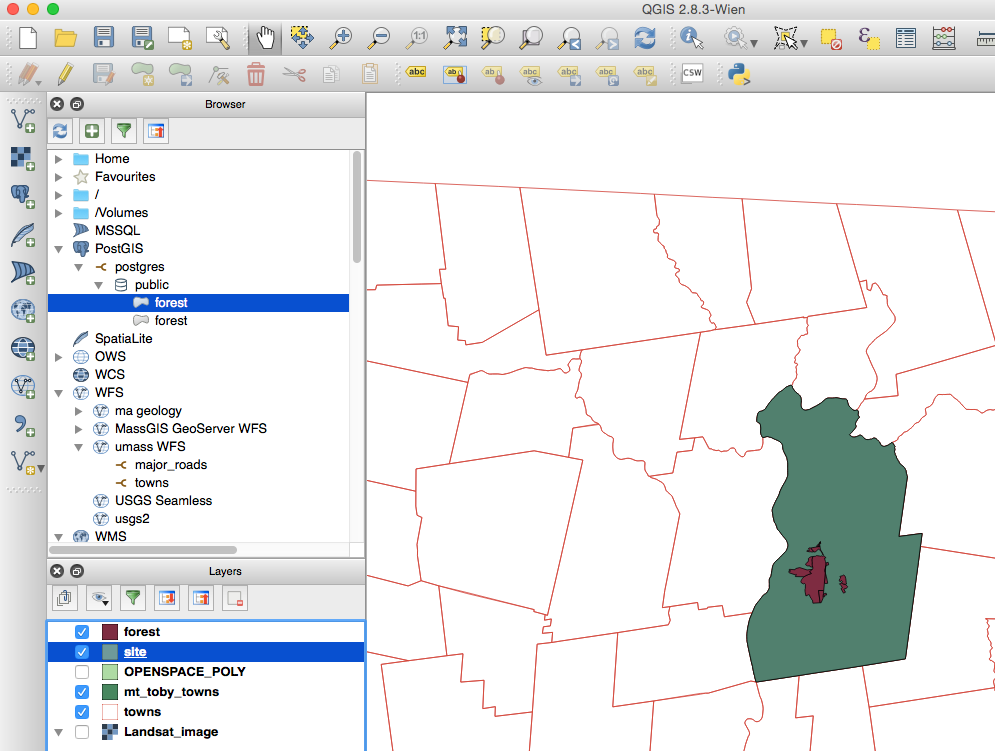
Now, to store that new Site shapefile in the IFRI PostGIS database, this is similar to what we did earlier using the QGIS Shapefile to PostGIS Import (SPIT) utility.

Next, add that new PostGIS layer to your QGIS Layers and map. This is similar to the steps we did in Answer 6 above, however you already should have the PostGIS connection to the IFRI database established in your QGIS Browser. So all you have to do is right click on the Public database under postgres, and click ‘refresh.’ The site layer should appear. Double click on that to bring that down to your Layers and to add it to your QGIS map. The CRS should be the same. Click OK.

Answer 7. Developing a random set of plot points within the mt toby forest boundary to create the ifri Plot table.

Use the Select by Expression tool to select out from the forest layer the polygon with GID = 10.
Layer, Save as ESRI Shapefile, Save as “study_forest” in your exercise folder, make sure you choose “Save only selected features.” OK. A new shapefile layer “study_forest” should appear in your list of Layers.

Now to create the random plot points…

QGIS Main menu, Vector, Research Tools, Random Points. See the parameters we used in the figure below:

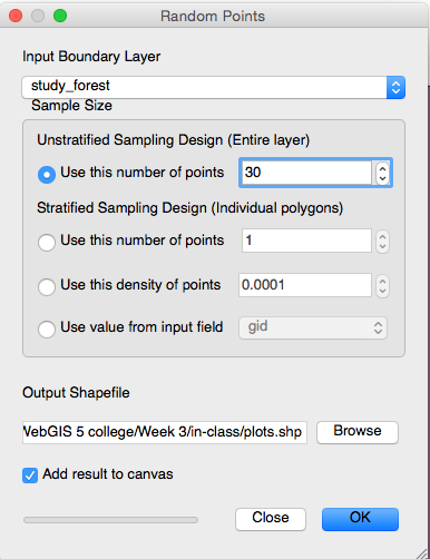
Press OK to run the random points function. Store it as Plots shapefile. Use the SPIT plugin utility to bring that into your IFRI PostGIS database and then add that layer to your QGIS Layer and map. Remove the old shapefile.

Answer 8. Add Plot_num (primary key), ForestID (foreign key) and Num_trees to the Plots table and enter some fake plots data.

Since Plots is a PostGIS layer, stored in a Postgres database, there are two ways you could do this: (1) in QGIS, or (2) using pgAdmin.

To do this in QGIS:

Select the plots table (highlight it in Layers)
Open up the attribute table (right click on plots, choose open attribute table, or press the table icon (figure A9.1) in the main icon menu at the top of QGIS)
Click on the “edit” icon at the top of the table screen
Click on the insert column icon at the top of the table screen

Add your columns using the above approach. All three fields could be defined as small integer.

Note that we already have a field called “gid” that could be used as the primary key for the plot points. But to be consistent with our relational database design, let’s create plot_num instead.

Once you have the columns created, enter some fake data:

plot_num, forestID, Num_trees

1,1,10

2,1,5

3,1,7

4,1,14

5,1,3

6,1,8

7,1,0

8,1,2

9,1,10

Note that all of these plots fall in the same forest, hence they all have the forestID “1”.

When done, press the “Save Edits” icon in the table menu (the little diskette) and then click the editor icon off. Close the attribute table.

NOTE: You could also have done this using pgAdmin!

Answer 9. Using pgAdmin’s Graphical Query Builder to query the IFRI database for all the Site, Forest and Plots records for Site 1

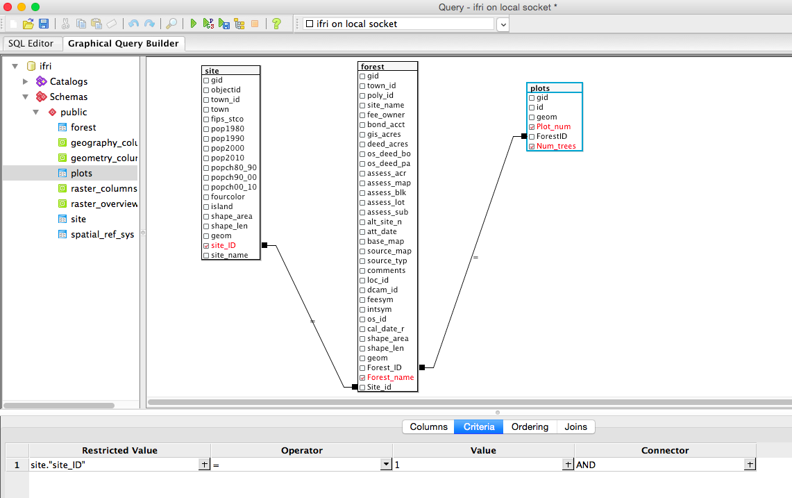
Pull the Site, forest and plots table into the graphical query area
Connect the tables using the primary and foreign keys you’ve set up to model the 1 to many relationships (e.g., Primary Site_id key in the Site table, to Site-id foreign key in the Forest table; also set up the relationship between Forest and Plots).
Select the fields (columns) you want returned in your query: site.site_id, forest.forestname, and plots.plot_num and plots.Num_trees. They should turn red when selected. See the below figure.
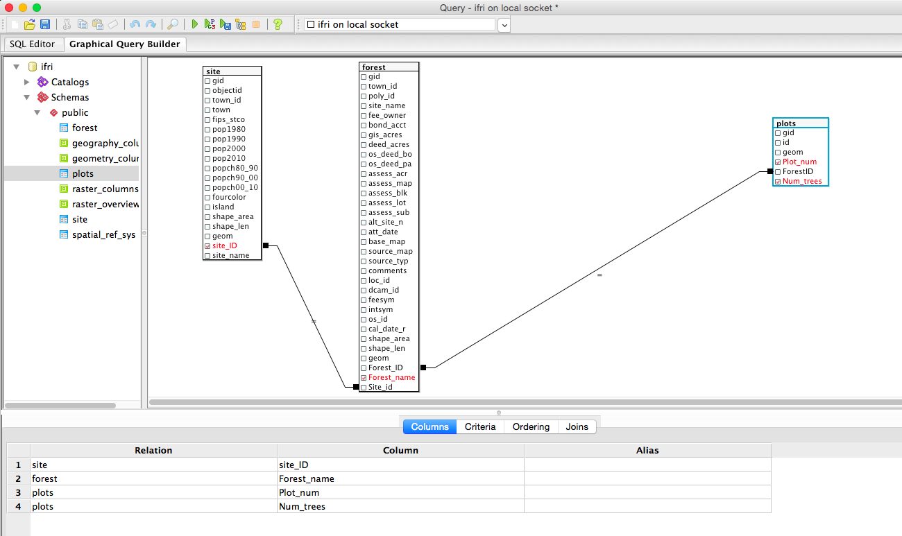
Now you have to do something you haven’t used yet in the Graphical Query Builder. Click on the “Criteria” tab at the bottom, and there you can enter the select criteria:

Restricted Value: site.site_ID

Operator: =

Value: 1

Your Query screen should look something like the figure below.

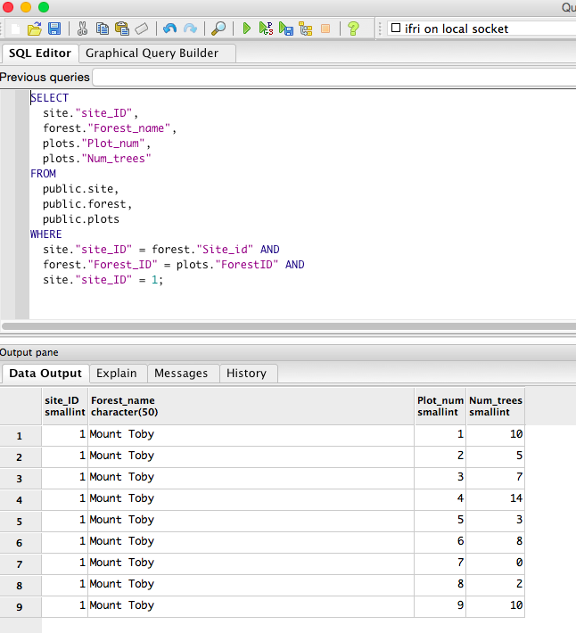
Run the query using the run query button (little green play icon). If successful, your results should look similar to the figure below, with the Site_ID data (“) from the Site table, the Forest_name (Mount Toby) from the Forest table, and the num_trees data from the Plots table.
Notice the SQL language that the Graphical Query Builder built.

Answer 10. How would you be able to list the plots that are in the forest boundary without using a 1-many relational database query?

In QGIS, use the Vector menu, Research Tools, Select by Location tool:

Select Features in “Plots” that intersect features in “forest”, creating new selection. OK.

You should see the plot points selected, and you can open up the plots table to see the results. If in this IFRI Forest polygon layer we had multiple forest boundaries, each with their own plots, we would have to do a more sophisticated query, asking first to select the forest boundary we want, and then doing the select by location query.

Building the IFRI Spatial Relational Database using PostGIS