Chapter 1. Exploring and Understanding Spatial Data Models

Lesson Goals

Students get an introduction to the desktop geographic information system software QGIS and learn how to access live data on the Internet using Web Mapping Services (WMS) and Web Feature Services (WFS).

Lesson Outcomes

Students can:

Use QGIS (the basics)
Connect to external data through WMS and WFS services
Distingush between WMS and WFS

Document Version: 10/17/2015

Revision author: Charles M. Schweik, UMass Amherst, and Andy Anderson, Amherst College

Attribution:

This material is based on earlier exercises developed by Kurt Menke GISP, Bird’s Eye View GIS, and Richard Smith, Ph.D.

Texas A&M University - Corpus Christi and offered through the GeoAcademy educational portal (http://fossgeo.org/free-qgis-courses/) and the Spatial {Query} Lab at Texas A&M Corpus Christi.

The development of the original document is funded by the Department of Labor (DOL) Trade Adjustment Assistance Community College and Career Training (TAACCCT) Grant No. TC-22525-11-60-A-48; The National Information Security, Geospatial Technologies Consortium (NISGTC) is an entity of Collin College of Texas, Bellevue College of Washington, Bunker Hill Community College of Massachusetts, Del Mar College of Texas, Moraine Valley Community College of Illinois, Rio Salado College of Arizona, and Salt Lake Community College of Utah. This work is licensed under the Creative Commons Attribution 3.0 Unported License. To view a copy of this license, visit http://creativecommons.org/licenses/by/3.0/ or send a letter to Creative Commons, 444 Castro Street, Suite 900, Mountain View, California, 94041, USA.

This document was original modified from its original form by Kurt Menke and continues to be modified and improved by generous public contributions.

Generic datasets used (other instructors can utilize their own site specific data by simply following these naming conventions in your data files):

TOWNS.shp (a polygon shapefile of towns and cities for a US state)

MAJOR_ROADS.shp (a line shapefile of major roads for a US state)

Landsat_image.tif (a Landsat image for the area)

Students: Before proceeding, download and unzip the Week 1 class data from the Moodle website.

Introduction

In this lab, students will explore and manage geospatial data using QGIS, an example of Free and Open Source for Geospatial (FOSS4G) software. It comes with two separate applications, QGIS Browser and QGIS Desktop. The former is an application analogous to Windows Explorer that is designed to preview and manage geospatial data, similar to ESRI’s ArcCatalog. QGIS Desktop is the companion application used to perform spatial analysis and make maps, similar to ESRI’s ArcMap.

Your Windows installation makes QGIS Desktop and QGIS Browser available with shortcuts on your desktop, but on Macs QGIS Browser is hidden inside of QGIS Desktop, which is probably in your folder Applications:

Right-click on QGIS.app and in its contextual menu select Show Package Contents.
Navigate to Contents/MacOS/bin/QGIS Browser.app.
Right-click on QGIS Browser.app and in its contextual menu select Make Alias.
Drag the alias into the folder Applications.

While it is sometimes useful to use QGIS Browser, this lab will instead focus on QGIS Desktop, and use its built-in Browser Panel.

For many students, this exercise will be simple and very intuitive, since QGIS operates very similar to other GIS software they may already be familiar with. This lab includes the following tasks:

Task 1 – Learn to work with QGIS Desktop.
Task 2 – Become familiar (or a brief refresher) with some common geospatial data models.
Task 3 – View traditional data stored on your local computer
Task 4 – View data available over the Internet through Web Mapping Service and Web Feature Services using QGIS Desktop.

We are assuming students have some experience with GIS coming into this course. If you do, you probably have used ESRI’s ArcGIS. For interested students, we are providing a couple of pretty recent links to comparisons done between ArcGIS and QGIS:

Most students taking this course will already know that Geographic Information Systems model the real world with representations of objects such as lakes, roads, and towns.

Geospatial data models are the means used to represent these features. They are composed to two parts: spatial features and attributes that when combined, create a model of reality.

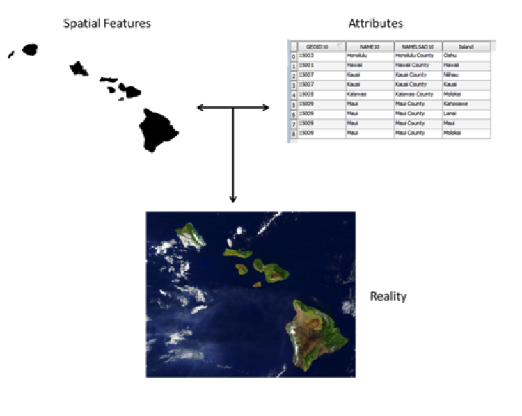Two parts of the geospatial data model

And as you also probably know, there are two main geospatial data models: vector and raster.

Vector Data Model – best for modeling discrete objects. Vector data comes in three basic forms: point, line, and polygon.

Raster Data Model – this model is best for modeling continuous objects. A raster is composed of a matrix of contiguous cells, with each cell (pixel) holding a single numeric value. Each value might represent reflected color as in a photograph, elevation in feet or meters, or other data.

Task 1 – Familiarize yourself with QGIS Desktop

In this task, you will become familiar with QGIS Desktop. The first step in working on a project with geospatial datasets is to organize your workspace. It is important that we organize datasets logically on the computer and make them easy to find. In this task, you will obtain a copy of the lab data and explore how the data is organized using the Browser Panel.

For this lab, we will explain how to open and use QGIS using the Mac Operating System and QGIS desktop version 2.8 (Wien).

Open QGIS Desktop. The way you open it will vary depending on your operating system.
The QGIS interface is simple and clean, with a large panel to display a map, several other panels, usually along the left side of the Map Panel, and a set of toolbars, usually positioned on the top and left.

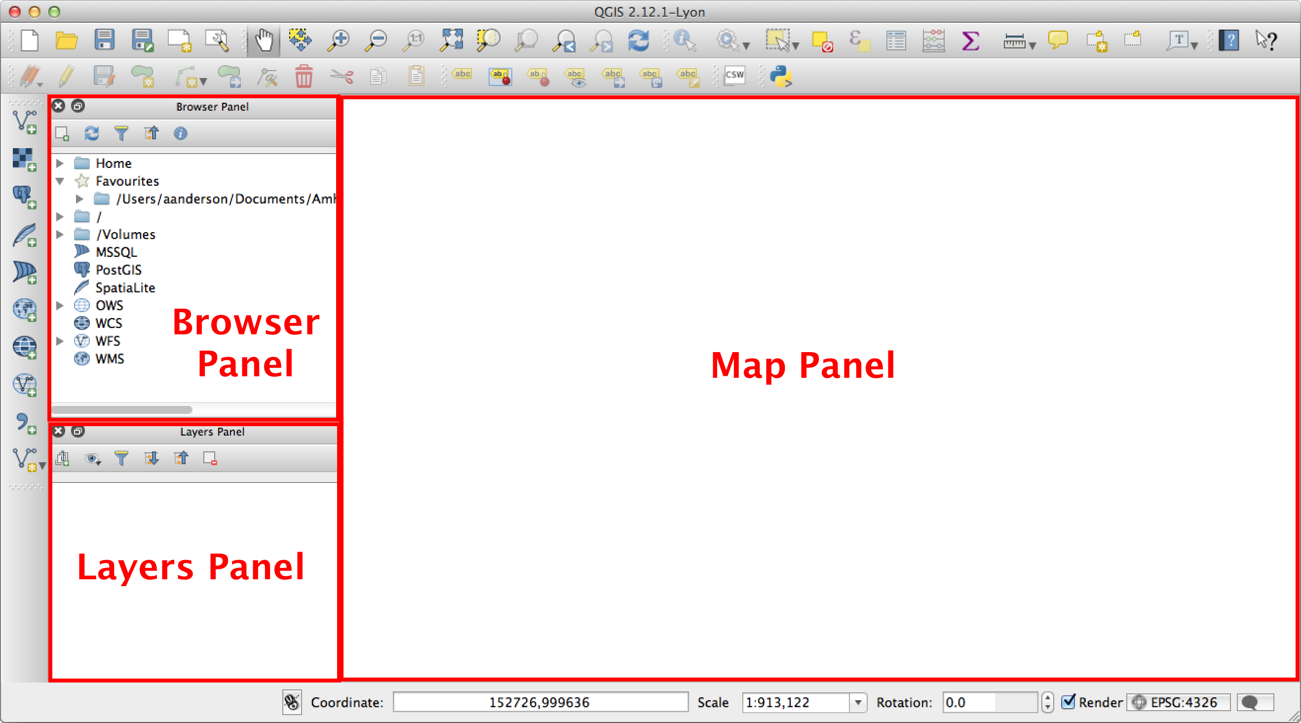QGIS Desktop

Any of the panels can be docked to and undocked from the QGIS Desktop window. To undock a panel, double-click its title bar (outlined in figure below), whence it will pop out of its location into a new window. You can also click and drag it away from the sides; when you release your mouse button, the panel will be floating freely.

Area to Double-Click or Drag When Undocking a Panel

To dock a floating panel, double-click its title bar, and the panel will return to its previous location. You can also drag it to the location where you want it, wait for the other panels to move out of the way to leave a gray space, and release.
To reset the QGIS Desktop window back to the default settings:
1. Menu Settings > Options;
2. In the dialog Options, click on the tab System;
3. In the section QSettings > Reset user interface to default settings (restart required), click on the button Reset;
4. Confirm by clicking the button OK, and QGIS Desktop will restart.
One of the panels is labeled Browser Panel. If it is not visible you can display it by menuing View > Panels > Browser Panel.

Within the Browser Panel, various sources of data are listed, beginning with the current project’s home folder (if you’ve saved it) and followed by your computer’s Home folder. Both can be expanded to show their files and folders by clicking on the buttons / and / at the left of each element.

These folders are followed by references to different drives and network drives or volumes. (NOTE: your machine may have a different set and number of drives listed here. This is fine.) Below the drives are various kinds of network database connections, which we will be learning about in next week’s material. There are no connections to any databases at this point.
In the Browser Panel, locate the lab folder where you stored your data (gisdata). Your browser might look something like the figure below.

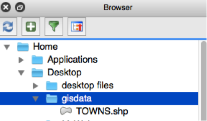
Lab Data in QGIS Desktop

Right-click on your data folder and select Add as a favourite, to provide quick access to it in the Browser Panel.

The icon indicates that the TOWNS dataset is a vector layer. The other common icon next to files, , is used to represent raster data but is also used for other files (such as XML files).

Task 2 - Become familiar with geospatial data models

Now that you are familiar with the basic layout of QGIS Desktop, we will explore some geospatial data that is stored on your local computer.

Let’s take a closer look at the layer TOWNS.shp currently listed in the Browser Panel in the data folder. To view its metadata, right click TOWNS.shp and in its contextual menu select Properties. The dialog Layer Properties will appear:

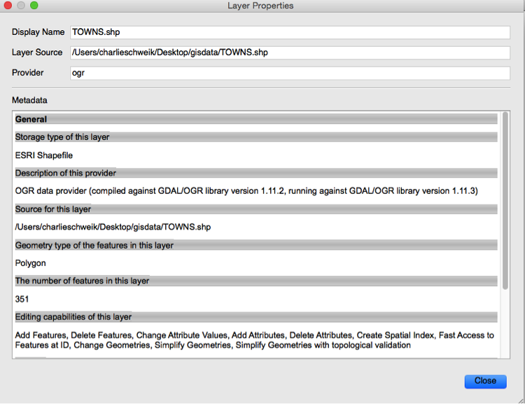Metadata in QGIS Desktop

In addition to data models (vector and raster) we have to understand file formats. Some file formats are designed to store vector data and others, raster data. Under Storage type of this layer we can see that it is an ESRI Shapefile, one type of vector file format. In fact they are (as of this writing) probably the most common vector file format – a proprietary format that has become a defacto-standard because it is so widely used. As you may know, a shapefile is actually a collection of files on the computer with a common name, but different extensions.

An individual shapefile can only contain one geometry type (polygon, line, or point). In this case, there are 611 polygons stored in this shapefile (many of the 351 Massachusetts cities and towns have disjoint islands, each one a separate polygon).

Also scroll down and note the Layer Spatial Reference System, which QGIS elsewhere refers to as the Coordinate Reference System (CRS). Although this layer is projected in NAD83 / Massachusetts State Plane Mainland, QGIS doesn’t provide that description, instead displaying the details of how the projection is constructed. Importantly, the linear unit is described by the phrase +units=m, meaning it is meters.
Now select MAJOR_ROADS.shp and view its properties. You’ll see that this is also an ESRI Shapefile but that it is a line dataset with 30 features.
Now, in the browser, right click on the dataset Landsat_image.tif, and look at its properties. It is a raster dataset in GeoTiff format, with 30-meter pixel resolution.
The QGIS Desktop interface is a little cluttered by default, so close any panels other than the Layers Panel and the Map Panel.

In particular, close the Browser Panel (which we used in the previous task), by clicking on the X button (on Windows in the upper right corner, on Macs in the upper left corner).

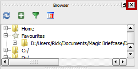
Close Browser Panel Button

Note: If you want to restore the Browser Panel (or other panels or toolbars), right click on any open gray space in any toolbar, e.g. to the right of the button What's This, and a contextual menu will appear.

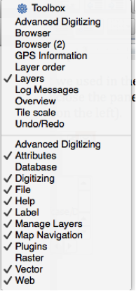
Select Browser and it will reappear.

With the QGIS Desktop interface customized, let’s add some data.

Task 3 - Viewing geospatial data in QGIS Desktop

Now that you know how geospatial datasets are stored on your computer, let’s see what the data they contain looks like.

You should still have QGIS Desktop open. If you don’t, invoke it again.

QGIS Desktop

Note the status information in the lower right corner describing the coordinate reference system (CRS) that is currently being used by QGIS, by default EPSG: 4326. This is the WSG 84 geographic CRS, which is one of roughly 2,700 known to QGIS. Its designation is from one of the two main CRS categorization systems that you will see referenced by QGIS, the European Petroleum Search Group (EPSG) and the Institut Géographique National de France (IGNF).

Like other geographic CRS, WSG 84 is displayed with a Plate Carrée projection, i.e. x = longitude and y = latitude.
QGIS has “Add Data” buttons for both vector and raster files, as well as for data sources such as databases and Internet map servers. These are located, by default, in the toolbar along the left side of the window.

Click the button Add Vector Layer.

Alternatively, you can menu Layer > Add Layer > Add Vector Layer….

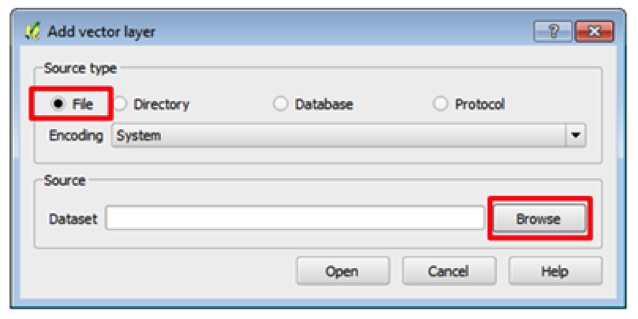
*Add Vector Layer Dialog*
The dialog Add vector layer will now appear. Let’s add one of the ESRI shapefiles, which is a file-based dataset. In the section Source type, click the button File. Then in the section Source, click the button Browse.
The dialog Open an OGR Supported Vector Layer will now appear. Navigate to your course data folder.

(Note: OGR is a FOSS4G project with the sole purpose to read and write geospatial vector data files. The meaning of OGR is historical. If you care, it used to stand for “OpenGIS Simple Features Reference Implementation.” For more information, you can read about it at http://trac.osgeo.org/gdal/wiki/FAQGeneral#WhatisthisOGRstuff.)

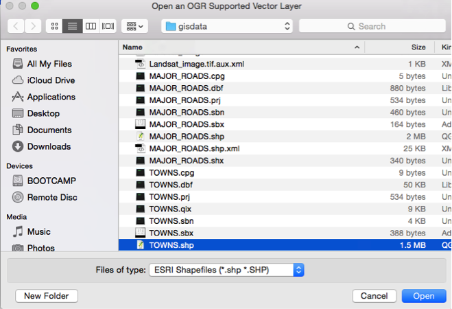
Open an OGR Supported Vector Layer

The file list defaults to all files, including several shapefiles in the course data folder.

But take a moment to see the other available file type options by clicking on the filter menu Files of type:. Did you know there were so many different types of geospatial data?

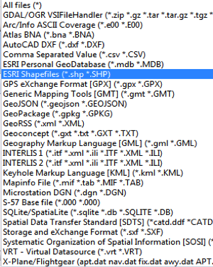
OGR Supported Vector Formats

After reviewing, select ESRI Shapefiles to see just that type of file.
Select TOWNS.shp and click the button Open.
Now back in the dialog Add vector layer, click the button Open to add the data to QGIS Desktop (see figure below).

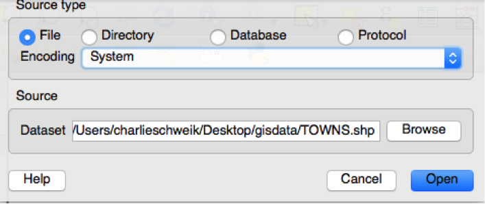
Add vector layer

You will now also see the layer TOWNS in the Layers Panel and the map features displayed in the Map Panel. Vector GIS layers will come in with random colors. You will learn how to change layer styling in a future exercise.

Also note that the displayed CRS has changed to USER: 100000. This is because QGIS has a default setting to use “on-the-fly” projection when a first layer is added whose projection is known. In this case, QGIS interprets the projection information in the shapefile’s .prj file, which is in Well-Known Text format, but doesn’t recognize it to be the same as EPSG 26986, NAD83 / State Plane Massachusetts Mainland (as we noted previously). It therefore assigns it a “User” designation.
Let’s examine the new layer’s attributes. In the Layers Panel, right-click on the layer TOWNS. In its contextual menu, select the menu item Open Attribute Table (shown in figure below).

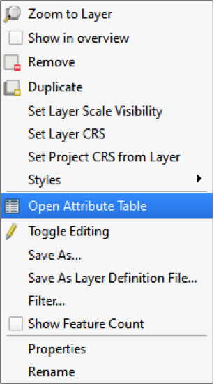
Layer Contextual Menu
The attribute table opens. If you recall from exploring this dataset with QGIS Browser, it has 351 features (351 polygons). The attribute table has 351 corresponding records. The table that appears will look similar to the figure below. As you may know, each row corresponds to one polygon. The columns are things we know about the polygons such as town name or its population for a certain year (see figure below).

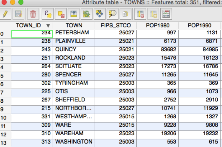Attribute Table
Close the Attribute Table by clicking the X button in the upper right hand corner.

As you may know from other GIS software experience, another way to interact with both the spatial features and the attributes is the Identify button.
Click the button Identify
Click on one of the features on the map. The Identify results panel (shown in figure below) shows you the attributes for the feature you clicked on. Note: The Identify results panel may initially be docked or floating.

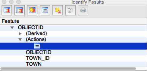
Identify Results

When you double-click on the little table icon under (Actions), it will bring you to the Feature Attributes window where you can see the attribute data for the feature you selected.

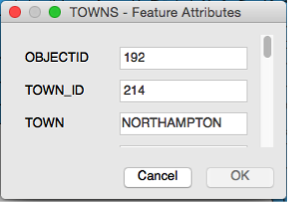
Identify Feature Attributes window

Now, let’s add Raster data to QGIS Desktop.
Click the button Add Raster Layer

Alternatively, click Layer | Add Layer | Add Raster Layer.
The Open a GDAL Supported Raster Data Source window opens (displayed in figure below). This is a very similar workflow to adding vector data.

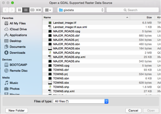
Open a GDAL Supported Raster Data Source
Whereas QGIS used OGR to open vector data files, here it uses another FOSS4G software library called GDAL. GDAL (sometimes pronounced “Gee-dall”) stands for “Geospatial Data Abstraction Library” is used for reading and writing raster datasets. In other words, it is a cross platform “translator library” that supports a variety of raster formats, such as “GeoTIFF, Erdase Imagine, SDTS, ESRI Grids, MrSID, JPG2000, etc.). “It is the primary data access engine for many applications including MapServer, GRASS, QGIS, and OpenEV. It is also utilized by packages such as OSSIM, Cadcorp SIS, FME, Google Earth, VTP, Thuban, ILWIS, MapGuide and ArcGIS. (source: http://www.osgeo.org/gdal_ogr)
The window’s raster data filter is set to All Files by default, so you see the entire contents of the folder (Figure below).

[GDAL] All Files
Open the “files of type” filter and see how many formats it will read! More than 50 different raster data formats! In GIS there are many more raster file types than vector.

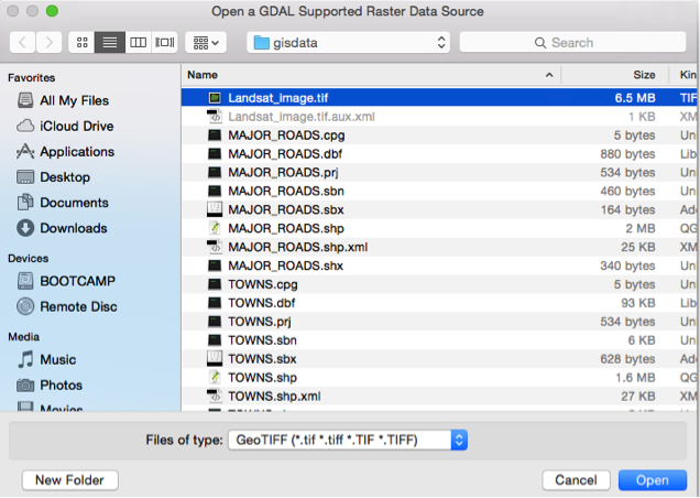
[GDAL] GeoTiff
Choose the raster dataset Landsat_image.tif and click the button Open.
Drag it to the bottom of the layer list and turn the fill color off on the Towns layer. Right click on TOWNS, Properties, Style, Click on Simple Fill, Fill down arrow, change to ‘Transparent Fill’. Set the Border to red. Hit OK. Your map screen should look similar to the below.

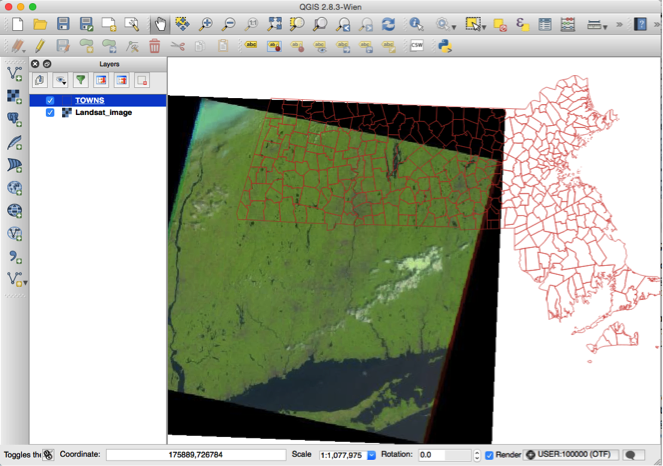
As you may know, this is an example of a raster dataset in QGIS. Like a photograph, it is composed of cells. This raster is a Landsat ‘true color’ satellite image of Western Massachusetts, Connecticut and extends all the way down to display a portion of Long Island. The image was taken on July 22, 2002.

If you don’t have the QGIS Browser panel open, open it (recall you can right click next to the help icon and select the Browser option. It will reappear). Scroll down the Browser panel and note the “Favourites” item.

Data is often stored deep inside a series of folders. It is often tedious and time consuming to navigate deep inside the folders to gain access to the data. Favourites provide a way to create a shortcut directly to any folder so that you have one-click access to any folder. Let’s create a favorite to our lab folder for practice.

Navigate to the lab data folder in the Browser panel. Right-click on it and choose Add as a Favourite (see figure below). Note: Currently this functionality is reserved only for the Browser tab in QGIS Desktop. However, once it is set it will show up as a Favourite in QGIS Browser as well.

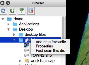
Add as a Favourite
Now expand Favourites and you will see your lab folder listed there. You can remove a favourite anytime by right-clicking on it and choosing Remove favourite. Note: You can drag data from the QGIS Browser application to QGIS Desktop as well to add the data to the map.

Task 4 - View data available over the Internet through Web Mapping Service and Web Feature Services using QGIS Desktop.

In the lecture portion of this first class, we discussed Web Feature Services and Web Map Services (WMS). Recall: A Web Feature Service (WFS) is a standard that allows the sharing of geographic map data at a feature level (i.e. sharing vector-based data such as ESRI Shapefiles (.shp)). This standard allows the user to request specified geographic data from a client and received the requested data via the web.

A Web Map Service (WMS): is a standard where geographic data can be displayed across the web and multiple platforms. This standard does not provide the actual geospatial data; instead it just provides a georeferenced image (e.g., PBG, JPEG or GIF) of the data. Utilizing WMS enables a user to access different geospatial databases without needing the original source data on local machines.

A variety of organizations provide live GIS data over the web as these kinds of services. In our state, the MassGIS organization is an important provider of data, and they offer these services.

Take a minute to read the overview of MassGIS Web Mapping Services and Applications page, available at:

https://wiki.state.ma.us/confluence/display/massgis/Overview+of+MassGIS+Web+Mapping+Services+and+Applications

MassGIS offers their data services through two different servers: (1) the proprietary ArcGIS Server, and (2) the open source GeoServer. It is the latter that we will use in this course.

Let’s try out MassGIS’ Web Mapping Service (WMS).

In the QGIS Browser, scroll down to where “WMS” is listed, and right click. You should see a “New Connection” option appear.
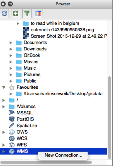
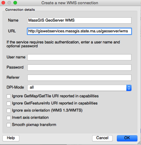
Give your WMS connection a name. In this case: “MassGIS GeoServer WMS”
Add the associated WMS URL. In this case: http://giswebservices.massgis.state.ma.us/geoserver/wms

Your screen should look like this:
Press OK
In the QGIS Browser, expand the WMS entry (press the little triangle) and you should see your new WMS entry listed, similar to the below.

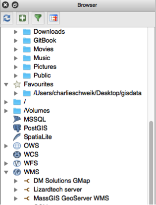
Click on the triangle next to “MassGIS GeoServer WMS” and it will attempt to connect to the MassGIS GeoServer. Eventually, you should see the below:

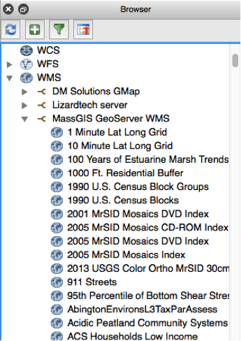
There are many, many layers you could choose to add to your QGIS map layers.

Suppose we were interested in identifying the watershed subbasin surrounding the Quabbin water supply – Boston’s water supply.

In the QGIS Browser, double click on the “Subbasins” option. In a few seconds (hopefully!) the approximately 2300 subbasin polygons will appear at the top of the Layers table of contents. Polygons will appear, although remember, this is a Web Map Service. If you look at the properties of this layer, you will see it is “singleband color data” – this is not a vector layer. It is rather, a “picture of the data.” Zoom into the area of the Quabbin as shown in the figure below.

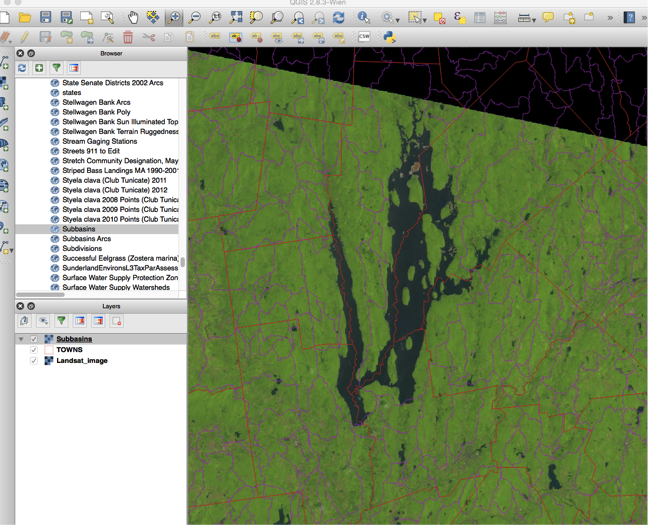
If you right click on the Subbasins raster entry, in the contextual menu you will see that there isn’t an attribute table to use. While the layer looks like a vector polygon layer, it is actually a raster file served using WMS via a GeoServer server over the Internet that is hosted by the MassGIS organization.

Now let’s try to connect to MassGIS’ Web Feature Service (WFS)

Recall that with a WFS, you are requesting to see the actual geographic features, rather than a picture of the data. That means you will be able to open the associated attribute table as well of this vector data.

In the QGIS Browser, close the long list of MassGIS data by slecting the triangle next to WMS. You should see the list go away or get minimized.
Right click on WFS in the QGIS Browser to bring up the “New Connection” contextual menu.
Enter a name such as "MassGIS GeoServer WFS" for name and "http://giswebservices.massgis.state.ma.us/geoserver/wfs" for the URL. Click OK. Your QGIS Browser should look similar to the below.
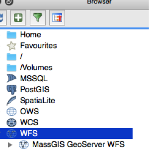
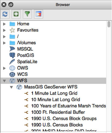
Click on the triangle next to the MassGIS GeoServer WFS entry. You will see it expand as shown in the Figure below:
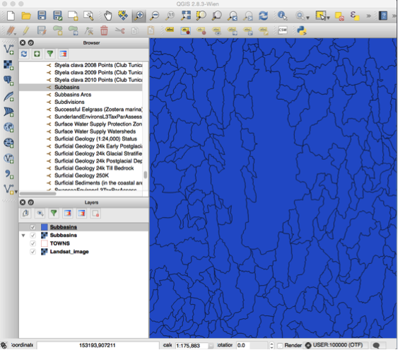
Scroll down the list and choose “Subbasins.” This brings up the same data as did our WMS exercise above, but in this case you are seeing the actual subbasin polygons. Your QGIS map screen should look something like the below:
If you right click on this entry in the Layers list, you will see the “Open Attribute Table” option --. Click it.
Because this is a “Web Feature Service”, these are vector polygons and its corresponding attribute table is available. You should see something like the below.
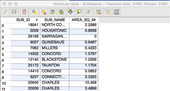
You can click on individual records in the left most column and their individual polygons will appear. For instance, if you are still zoomed in around the Quabbin Reservoir click on one of the “Chicopee” entries and you should see one of those associated subasins selected.

Note that there are many Web Mapping and Feature Mapping Services available these days!

For example, try and connect to one or more of the USGS Web Mapping Service options listed on their Seamless website:

http://seamless.usgs.gov/services.php

It takes some sleuthing to find the correct URL to use for the WMS. For example, try out the National Land Cover Database 2011 map service. See if you can find this link in the extensible markup language (XML) file they provide for WMS:

http://isse.cr.usgs.gov/arcgis/services/LandCover/USGS_EROS_LandCover_NLCD/MapServer/WmsServer?

Add that WMS connection and see if you can get it operational in QGIS or try another option, such as the USGS Geologic Map data. For example, in the Figure below, we are displaying Massachusetts’ fault lines via a USGS WFS.

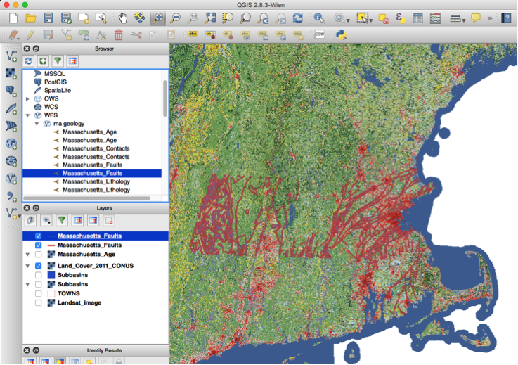
See this page for more on that available data: http://mrdata.usgs.gov/geology/state/state.php?state=MA

The specific WMS link is: http://mrdata.usgs.gov/services/ma?service=WMS&version=1.1.1&request=GetCapabilities

Or, the WFS version: http://mrdata.usgs.gov/services/ma?service=WFS&version=1.0.0&request=GetCapabilities

If time permits, take some time to see if you can find other WMS or WFS services on the web for the USA or for Massachusetts specifically and see if you can get it operational on your QGIS system.

Now let’s try to connect to our class Web Mapping Service (WMS) and our Web Feature Service (WFS)

To finish up this exercise, now let’s access our Landsat data and our towns layer using our own class WMS and WFS. This uses our own Geoserver which we will talk about in a future class.

Connect to our class WMS and look at the Landsat and towns layer using this service

To do this, you need to create another new WMS connection in your QGIS browser. The information you need is the following:

Name: UMass WMS URL: http://nrcwg01.eco.umass.edu:8080/geoserver/wms

Once you connect to the above, you should see in your QGIS browser a new entry under WMS for the UMass WMS server. Below that, you should see an entry for "Landsat_image" and also for the "Towns".

Click on these and load them into your QGIS map. The Landsat image should look the same as before other than it is stored on a server instead of your own local hard drive. The Towns layer should look, maybe, different. How?

With a little sleuthing, you may notice that while it looks like a vector layer, it isn’t. It is an image that displays that vector layer. So you can’t change the fill color or make it no fill. You are stuck with it “blanketing” over the Landsat image. That’s the difference, again, between a WMS service and a WFS service.

Connect to our course map server

Now let’s try and get the towns layer using our own class server’s WFS.

In the QGIS browser, create a new WFS connection.

To set it up, you need the following information:

Name: UMass URL: http://nrcwg01.eco.umass.edu:8080/geoserver/wfs

Once the connection is made, you should see two layers below the umass WFS: major_roads and towns.

Click on the towns layer and it should eventually appear in your QGIS map screen. But change the properties and turn off the fill. Notice you can also open the attribute table.

Do you want more on the specific operations of QGIS? There is a good set of tutorials available at:

http://docs.qgis.org/2.8/en/docs/training_manual/

We encourage you to do more on your own, especially if you feel you need it!

Task 5 – Upload a screenshot of your QGIS screen to Moodle

To complete this exercise, take a screen shot of your QGIS screen and upload it in Moodle under Week 1’s turn-it-in Exercise 1 option to get credit for this exercise.

Conclusion

In this exercise you explored datasets that use the two common geospatial data models: vector and raster. You have also used the QGIS Browser to preview datasets and in particular, you worked with some externally served data using Web Mapping Services and Feature Mapping Services, often served by an external server called “GeoServer.”

Exploring Spatial Data Models using QGIS